STA 302H1F / 1001HF -- Methods of Data Analysis I
-- Fall 2010
SAS examples from lecture:
CFCs on Mauna Loa example:
Data:
Data January 1977 to December 1993 (text)
Data December 1994 to December 2004 (text)
Analysis comparing means before and after the Montreal Protocol using the t-test (why isn't this analysis appropriate?):
SAS code (text)
SAS output (.lst) (text)
Linear regression analysis:
SAS code (text)
SAS log (text)
SAS output (.lst) (text)
Plot of CFCs vs time (pdf)
Before the Montreal Protocol: Plot of CFCs vs time with regression line (pdf)
Before the Montreal Protocol: Plot of residuals versus time (pdf)
Before the Montreal Protocol: Plot of residuals versus predicted values (pdf)
Before the Montreal Protocol: Plot of standardized residuals versus predicted values (pdf)
Before the Montreal Protocol: Normal quantile plot of residuals (pdf)
Before the Montreal Protocol: Normal quantile plot of standardized residuals (pdf)
After the Montreal Protocol: Plot of CFCs vs time with regression line (pdf)
After the Montreal Protocol: Plot of residuals versus time (pdf)
After the Montreal Protocol: Plot of residuals versus predicted values (pdf)
After the Montreal Protocol: Plot of standardized residuals versus predicted values (pdf)
After the Montreal Protocol: Normal quantile plot of residuals (pdf)
After the Montreal Protocol: Normal quantile plot of standardized residuals (pdf)
Anscombe example (4 made-up datasets):
SAS code (including data) (text)
SAS output (text)
Scatterplot of y1 vs x1 (pdf)
Scatterplot of y2 vs x1 (pdf)
Scatterplot of y3 vs x1 (pdf)
Scatterplot of y4 vs x2 (pdf)
Scatterplot of y1 vs x1 with regression line (pdf)
Scatterplot of y2 vs x1 with regression line (pdf)
Scatterplot of y3 vs x1 with regression line (pdf)
Scatterplot of y4 vs x2 with regression line (pdf)
Smoking and cancer example:
Data (text)
SAS code (text)
SAS output (.lst) (text)
Scatterplot (pdf)
Scatterplot with regression line (pdf)
Plot of residuals versus smoking index (pdf)
Plot of residuals versus predicted values (pdf)
Crime and population example:
SAS code (including data) (text)
SAS output (text)
Scatterplot of Number of violent crimes vs Population (all data points) (pdf)
Scatterplot of Number of violent crimes vs Population (all data points) with regression line (pdf)
Scatterplot of Number of violent crimes vs Population with regression line with New York City deleted (pdf)
Scatterplot of Number of violent crimes vs Population with regression line with New York City, Boston and Washington deleted (pdf)
Non-technical description of analyses including and not including New York (text)
SAS code with simple option on proc reg
SAS output with simple option on proc reg
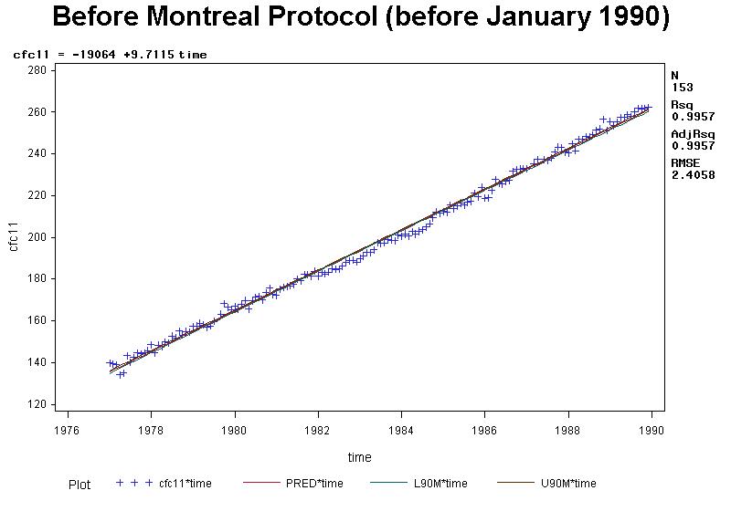
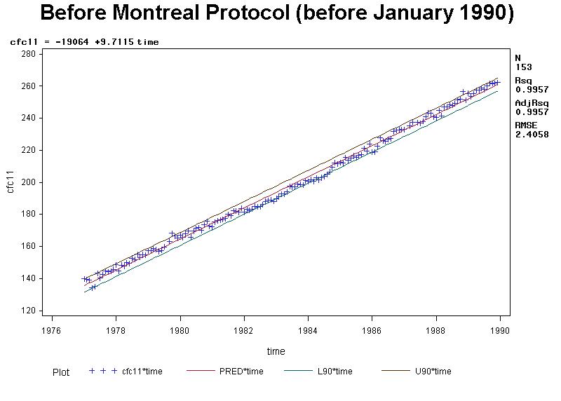
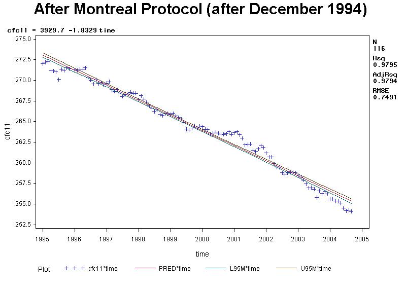
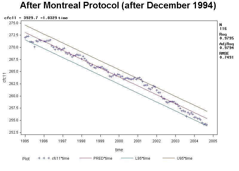
CFCs example with confidence and prediction intervals:
SAS code (text)
SAS output (text)
Plot of confidence intervals for mean of Y, pre Montreal Protocol (jpg)
Plot of prediction intervals for Y, pre Montreal Protocol (jpg)
Plot of confidence intervals for mean of Y, post Montreal Protocol (jpg)
Plot of prediction intervals for Y, post Montreal Protocol (jpg)
Plots of confidence and prediction intervals for smoking and cancer example:
Plot of confidence intervals for mean of Y (pdf)
Plot of prediction intervals for Y (pdf)
Normal quantile plots for simulated data (for Chapter 3):
Data are random sample of size 10 from standard normal distribution
Data are a second random sample of size 10 from standard normal distribution
Data are random sample of size 50 from standard normal distribution
Data are random sample of size 100 from standard normal distribution
Data are random sample of size 100 from t distribution with 2 df (heavy tails)
Data are random sample of size 100 from chisquare distribution with 10 df (right-skewed)
Crime example residual plots (for Chapter 3):
Residuals versus predicted values plot (pdf)
Studentized residuals versus predicted values plot (pdf)
Normal quantile plot of residuals (pdf)
Normal quantile plot of standardized residuals (pdf)
Crime example with influence statistics:
SAS code (text)
SAS output (text)
Corrosion example (for Chapter 3):
SAS code (including data) (text)
SAS output (text)
Scatterplot with regression line (gif)
Plot of standardized residuals versus predictor variable (gif)
Plot of standardized residuals versus fitted values (gif)
Normal quantile plot of standardized residuals from proc reg (gif)
Sequence plot of standardized residuals (gif)
Plot of square root of absolute value of standardized residuals versus fitted values (gif)
Breakdown example (for Chapter 3):
SAS code (text)
Data (text)
SAS output file (text)
Scatter plot for untransformed data with regression line (pdf)
Residuals versus X plot for untransformed data (pdf)
Studentized (standardized) residuals versus X plot for untransformed data (pdf)
Residuals versus predicted values plot for untransformed data (pdf)
Normal quantile plot of residuals for untransformed data (pdf)
(Residuals here have not been standardized but resulting plot would be similar.)
Scatter plot for data with square root of Y with regression line (pdf)
Studentized residuals versus X plot for data with square root of Y (pdf)
Residuals versus predicted values plot for data with square root of Y (pdf)
Normal quantile plot of residuals for data with square root of Y (pdf)
(Residuals here have not been standardized but resulting plot would be similar.)
Scatter plot for data with log of Y with regression line (pdf)
Studentized residuals versus X plot for data with log of Y (pdf)
Residuals versus predicted values plot for data with log of Y (pdf)
Normal quantile plot of residuals for data with log of Y (pdf)
(Residuals here have not been standardized but resulting plot would be similar.)
Scatter plot for data with 1/Y with regression line (pdf)
Studentized residuals versus X plot for data with 1/Y (pdf)
Residuals versus predicted values plot for data with 1/Y (pdf)
Normal quantile plot of residuals for data with 1/Y (pdf)
(Residuals here have not been standardized but resulting plot would be similar.)
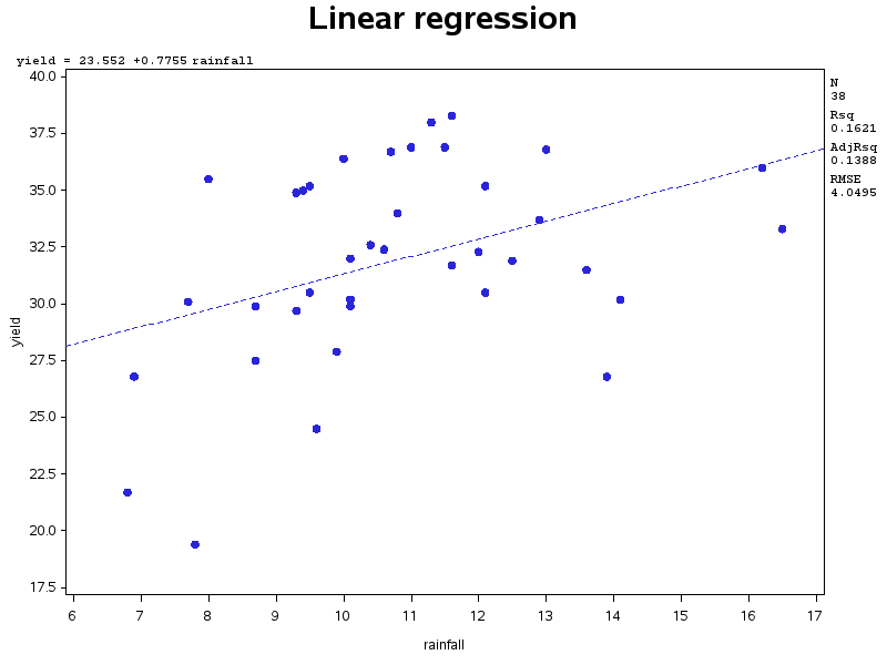
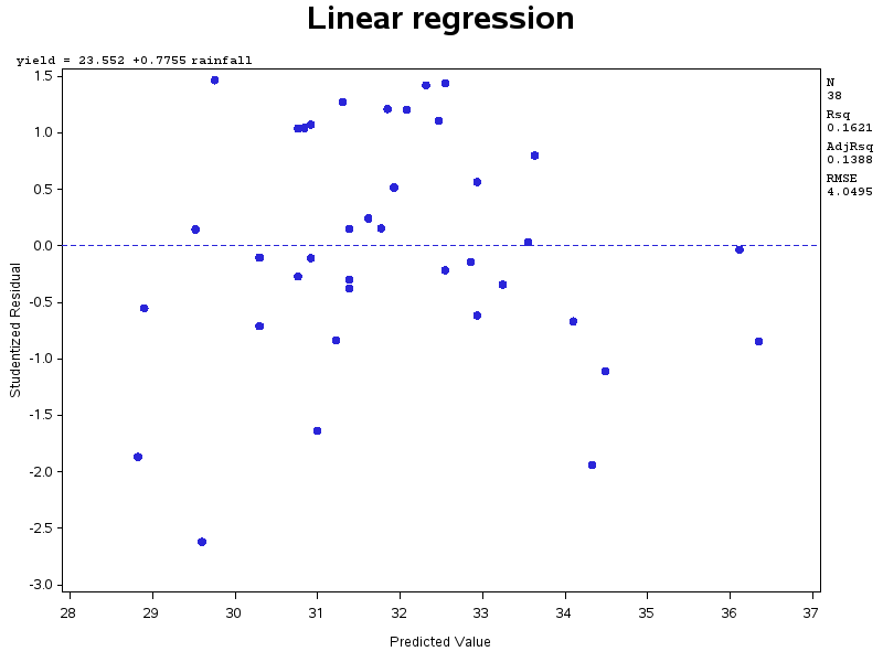
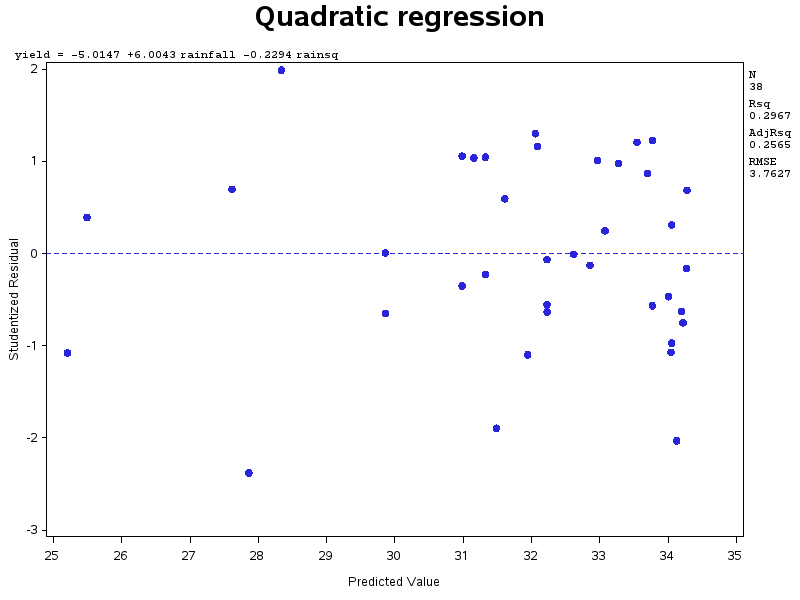
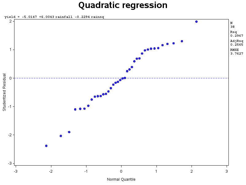
Rainfall and corn yield (Chapter 5):
Data (text)
SAS code (text)
SAS output (text)
Scatterplot of yield versus rainfall with simple regression line (png)
Plot of standardized residuals versus predicted values for simple regression (png)
Plot of standardized residuals versus predicted values for quadratic regression (png)
Normal quantile plot of standardized residuals for quadratic regression (png)
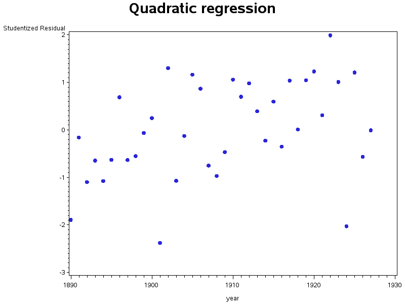
Plot of standardized residuals versus year for quadratic regression (png)
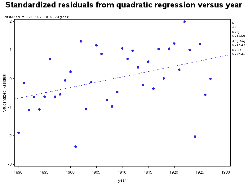
Plot of standardized residuals versus year for quadratic regression with regression line added (png)
CFCs on Mauna Loa example, quadratic regression:
SAS code (text)
SAS output (text)
Meadowfoam experiment (indicator variables and the partial F test (Chapter 5):
Data (text)
SAS code (text)
SAS output (text)
More on the meadowfoam example (ANCOVA (Chapter 5)):
SAS code (text)
SAS output (text)
Plot of number of flowers per plant versus light intensity, coded for timing (pdf)
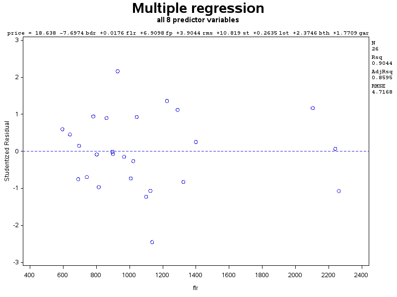
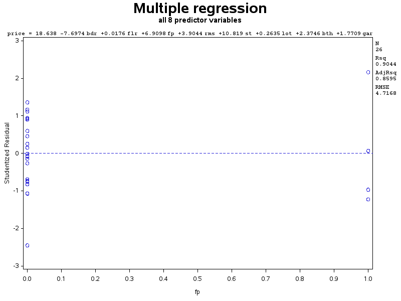
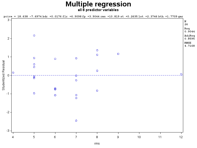
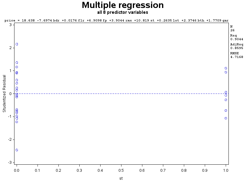
Chicago house sales example (for Chapter 6):
Data (text)
SAS code (text)
SAS output (text)
Pairwise scatterplots of all variables (pdf)
Residual plots:
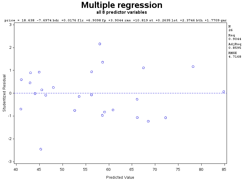
Standardized residuals versus predicted values (png)
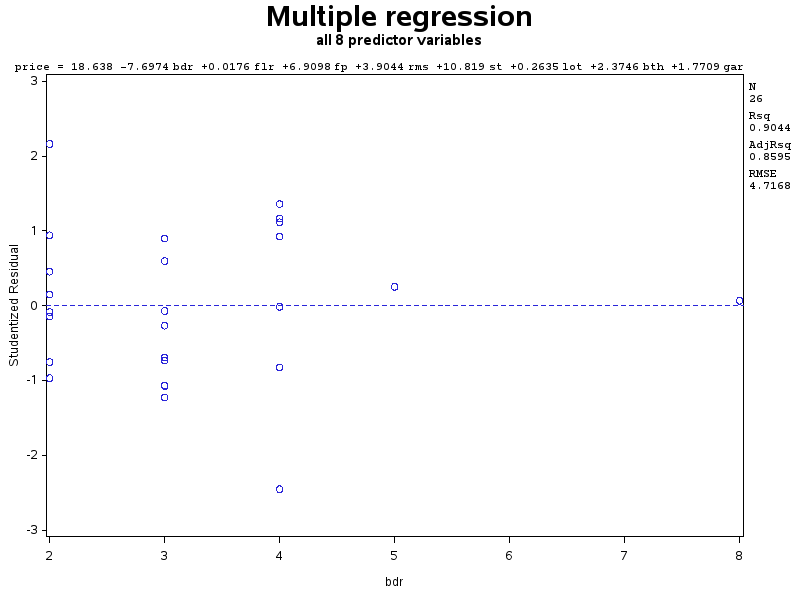
Standardized residuals versus number of bedrooms (png)
Standardized residuals versus floor space (png)
Standardized residuals versus number of fireplaces (png)
Standardized residuals versus number of rooms (png)
Standardized residuals versus indicator for storm windows (png)
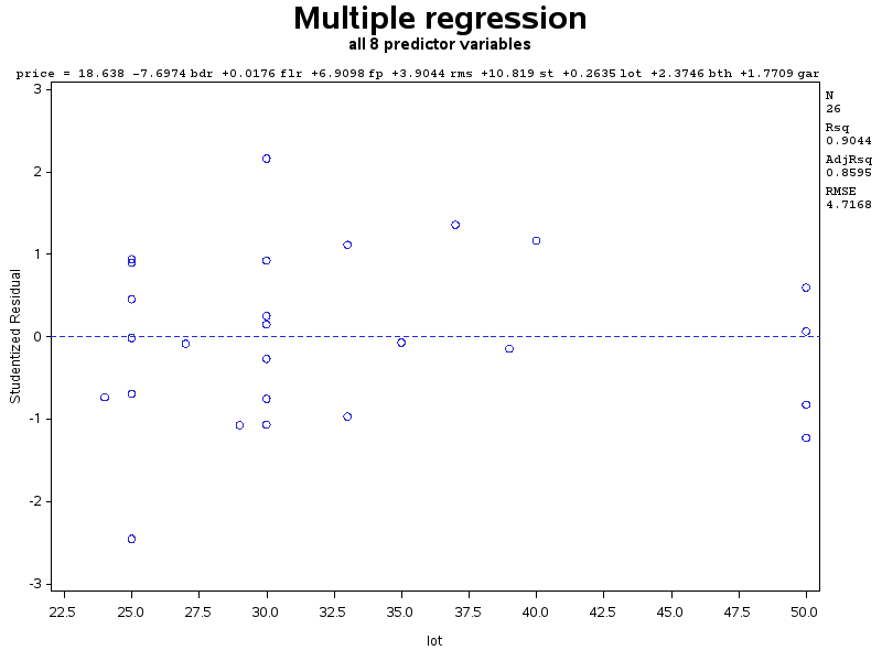
Standardized residuals versus lot size (png)
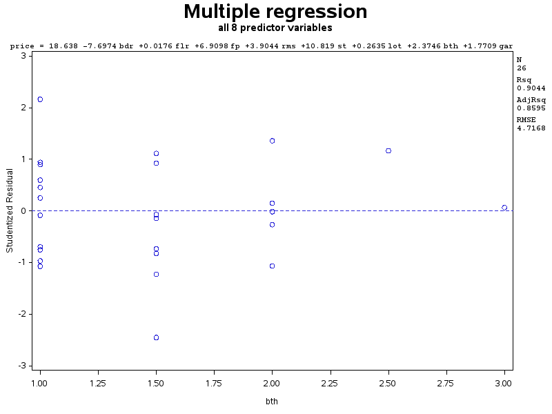
Standardized residuals versus number of bathrooms (png)
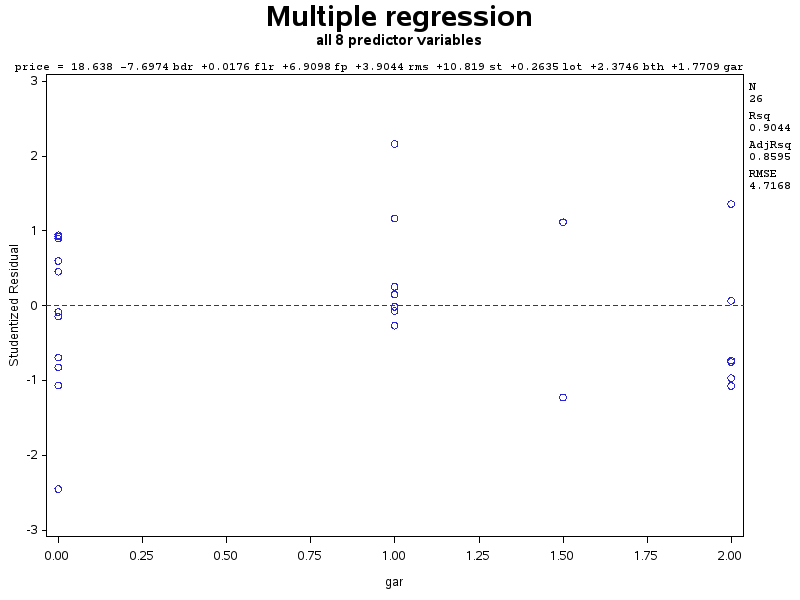
Standardized residuals versus number of garage spaces (png)
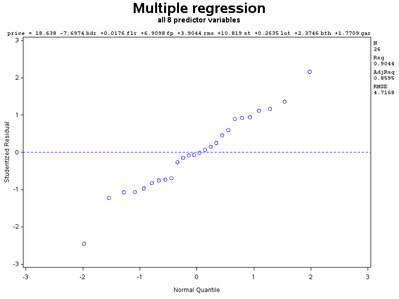
Normal quantile plot of standardized residuals (png)
Added variable plots:
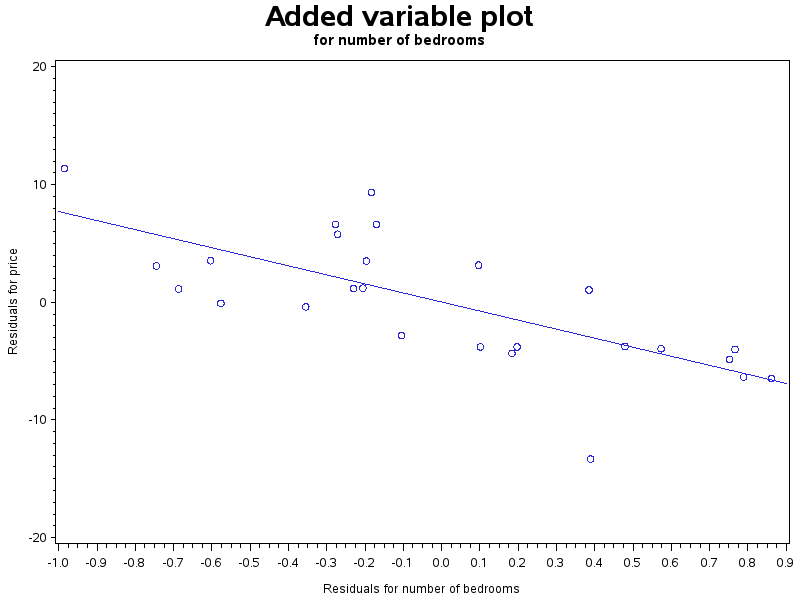
Added variable plot for number of bedrooms (png)
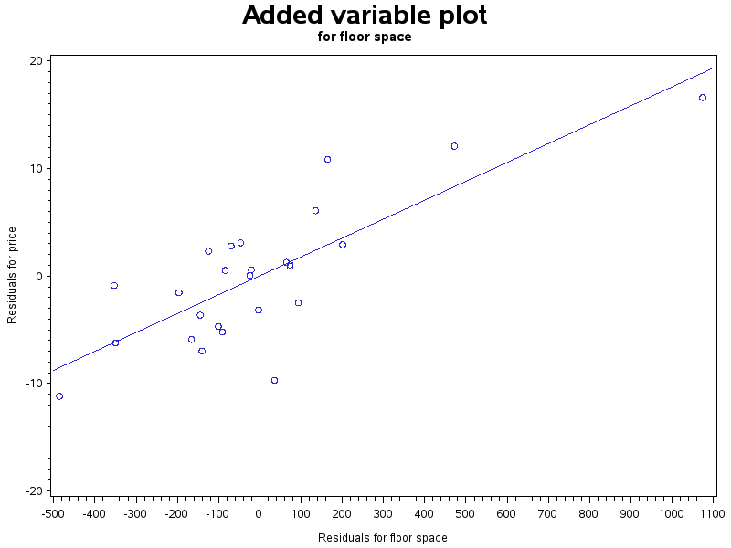
Added variable plot for floor space (png)
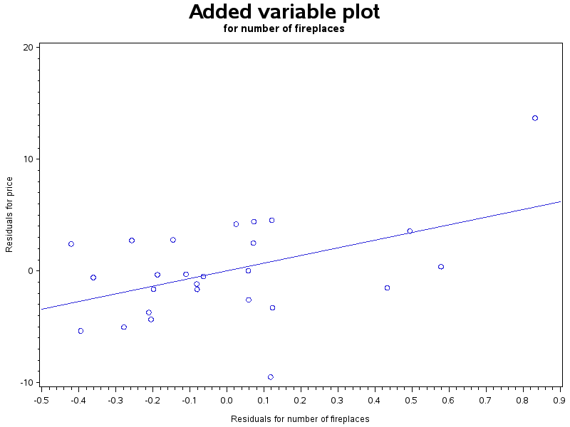
Added variable plot for number of fireplaces (png)
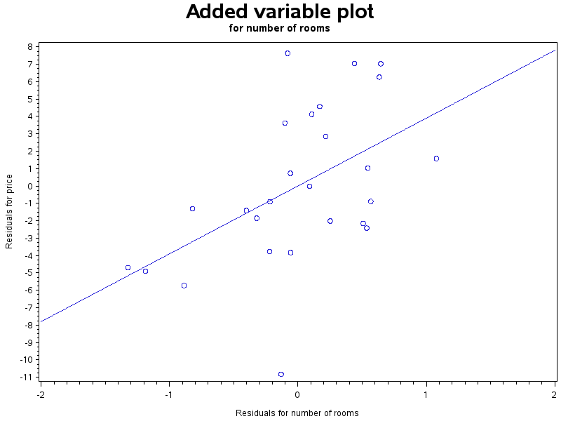
Added variable plot for number of rooms (png)
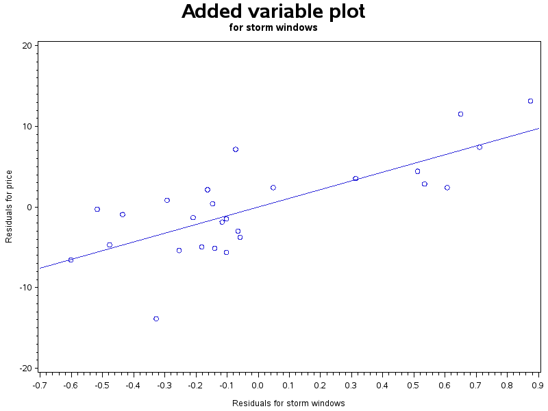
Added variable plot for storm windows (png)
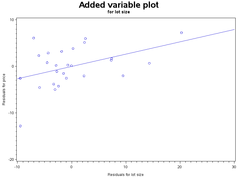
Added variable plot for lot size (png)
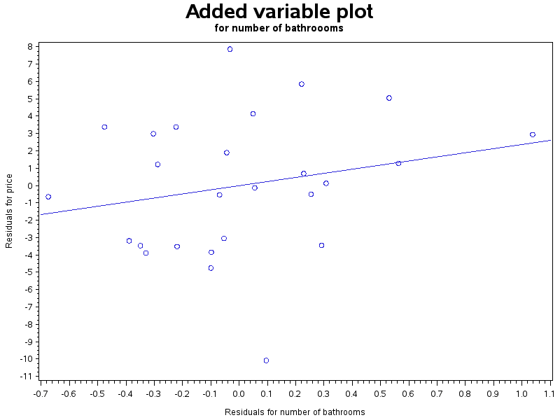
Added variable plot for number of bathrooms (png)
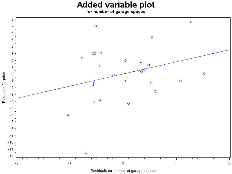
Added variable plot for number of garage spaces (png)